LLM Scaling Laws Paper Excerpt - Scaling Laws for Neural Language Models
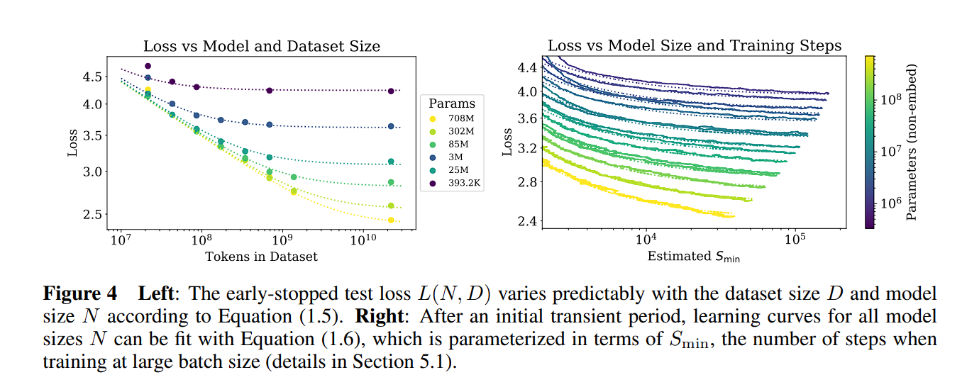
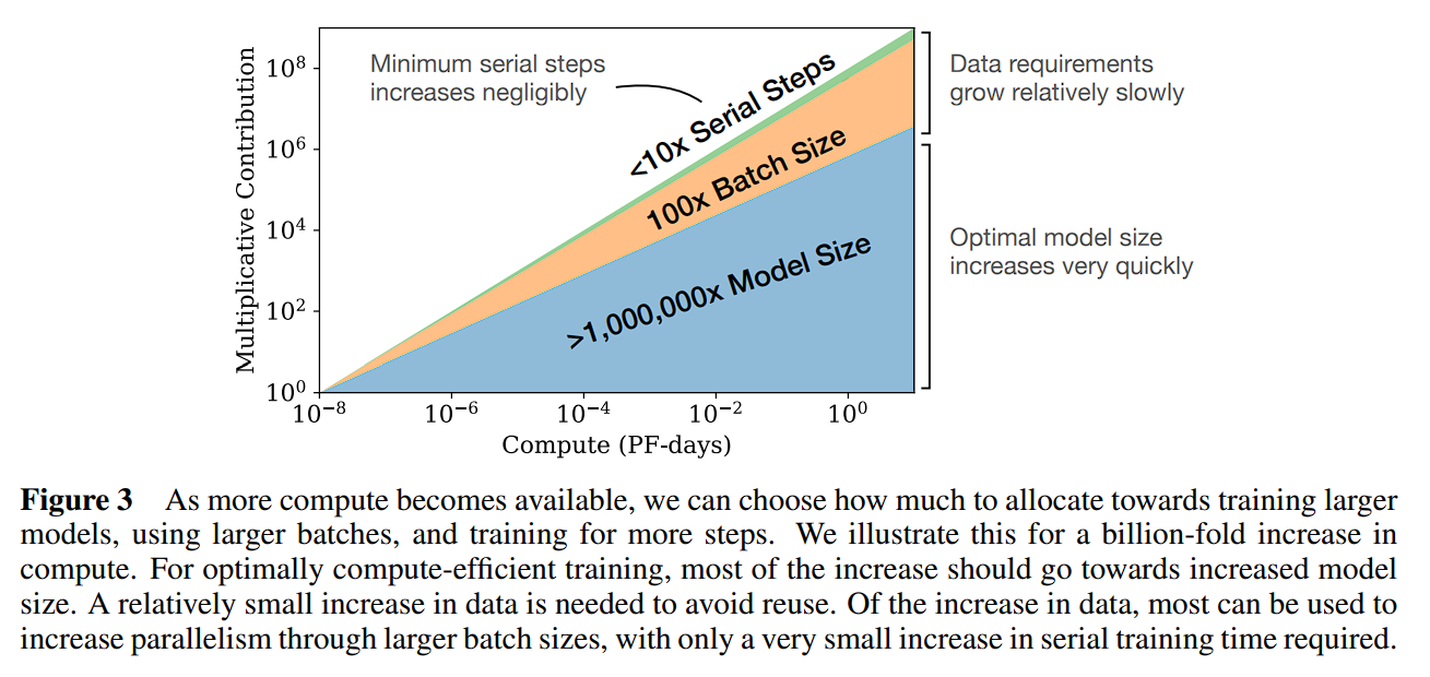
LLM Scaling Laws Paper Excerpt - Scaling Laws for Neural Language Models type: Post status: Published date: 2024/03/20 tags: AI, LLM, NLP, 论文摘录 category: 技术分享 In 2020, OpenAI released the paper “Scaling Laws for Neural Language Models,” exploring Scaling Laws. This paper discusses the relationship between the training loss of large models based on Transformers and the model parameter size (N), dataset size (D), and computational volume (C). In April 2022, Google DeepMind revisited Scaling Laws in their article “Training Compute-Optimal Large Language Models.” They pointed out that current large models are significantly under-trained. By using four times the data (compared to the 280B parameter Gopher) to train the 70B parameter Chinchilla, they achieved better results (SOTA average accuracy of 67.5% on the MMLU benchmark, a 7% increase). However, in February 2023, a blog titled “Chinchilla’s Death” by Thaddée Tyl argued that with sufficient training time, small models can outperform large models. This figure illustrates the contributions of different factors under the same compute budget (C). Firstly, model size contributes the most, followed by data (achieved through larger batch sizes and reduced data reuse), while increasing the number of serial steps (more training iterations) does not significantly help. Parameters: non-embedding parameters $N$ the dataset size $D$ optimally allocated compute budget $C_{min}$ When the other two factors are not limited, the test loss can be predicted using the following formula: $$ \begin{equation} L(N)=(N_c/N)^{\alpha_N} \end{equation} $$ \alpha_N \sim 0.076,N_c \sim 8.8 \times 10^{13} \text{(non-embedding parameters)} $$ $$ \begin{equation} L(D)=(D_c/D)^{\alpha_D} \end{equation} $$ $$ \alpha_D \sim 0.095, D_c \sim 5.4 \times 10^{13}\text{(tokens)} $$ $$ \begin{equation}L(C_{min})=(C^{min}c/C{min})^{\alpha_{min}} \end{equation} $$ $$ \alpha_C^{min} \sim 0.050, C^{min}_c \sim 3.1 \times 10^8 \text{(PF-days)} $$ Formula Meaning: In the above formulas, $\alpha_N, \alpha_D, \alpha_C^{min}$ indicate the power law exponents that describe the performance improvement when increasing $N,D,C_{min}$. For example, if we double the number of model parameters, the model loss will decrease by a factor of $2_{-\alpha_N}\approx 0.95$, meaning the loss will be 0.95 times the previous value. The exact numbers for $N_C,D_C,C_C^{min}$ are based on vocabulary size and tokenization, thus only representing an order of magnitude relationship rather than precise values. Additionally, the paper discusses the relationship between batch size and loss. $$ \begin{equation}B_{crit}(L)=\frac{B_*}{L^{1/a_B}} \end{equation} $$ $$ B_* \sim 2\cdot10^8 \text{tokens}, \alpha_B\sim0.21 $$ Based on the previous formulas (1) and (2), when we increase the model size, we should correspondingly increase the dataset size. It can be calculated as:$D\propto N^{\frac{\alpha_{N}}{\alpha_D}} \sim N^{0.74}$。 They also derived a combined formula from (1) and (2) to manage the dependencies of N and D and to control overfitting: $$ \begin{equation}L(N,D)=\left[\left(\frac{N_c}{N}^{\frac{\alpha_N}{\alpha_D}}+\frac{D_c}{D} \right) \right]^{\alpha_D}\end{equation} $$ The training curve can also be derived from the number of training steps, allowing us to determine the optimal number of training steps. $$ \begin{equation}L(N,S)=\left(\frac{N_c}{N}\right)^{\alpha{N}}+\left(\frac{S_c}{S_{min}(S)}\right)^{\alpha_S}\end{equation} $$ $S_c \approx 2.1 \times 10^3,\alpha_S \approx 0.76$ $S_{min}(S)$ is the minimum possible number of optimization steps (parameter updates) estimated using Equation In the case of fixed compute C, the following relationship formula is derived: $$ \begin{equation}N \propto C^{\alpha^{min}_C /\alpha_N}, B \propto C^{\alpha^{min}_C /\alpha_B}, S \propto C^{\alpha^{min}_C /\alpha_S}, D = B \cdot S\end{equation} $$ Here we have: $$ \begin{equation}\alpha^{min}_C=1/(1/\alpha_S+1/\alpha_B+1/\alpha_N)\end{equation} $$ So we can get $N \propto C^{0.73}{min}, B \propto C^{0.24}{min},\text{ and }S \propto C^{0.03}_{min}$,here drop out the ideas: When the compute budget C is increased, it should primarily be used to create larger models rather than extending training time or increasing dataset size. Additionally, as models become larger, they become more sample efficient. The study was conducted using the WebText2 dataset and its extension (2.29 × 10^10 tokens). The tokenization method employed was byte-pair encoding, with a vocabulary size of $n_{vocab}=50257$. The performance metric (Loss) was the cross-entropy loss over a context of 1024 tokens. The primary model used was a decoder-only Transformer, and LSTM along with other types of Transformers were also trained for comparison. Unless otherwise specified, the model training utilized the Adam optimizer for $2.5 \times 10^5$ steps with a batch size of 512 and a context of 512 tokens. Due to memory constraints, the largest models were trained using the Adafactor optimizer. The learning rate schedule, unless otherwise noted, included a warm-up period of 3000 steps followed by cosine decay to zero. Model Parameter Calculation Method To calculate the model parameters and compute requirements, the model hyperparameters are defined as follows: $N$ to represent the size of the model parameters, excluding the embedding layers, the calculation for model parameters is as follows: $$ \begin{aligned} N&\approx 2d_{model}n_{layer}(2d_{attn}+d_{ff}) \ &= 12n_{layer}d^2_{model}\end{aligned} $$ $$ d_{attn}=d_{ff}/4=d_{model} $$ Here, the parameters for the embedding layers $n_{vocab}d_{model}$ and $n_{ctx}d_{model}$ are omitted. The compute required for a forward pass, denoted as $C$, is approximately: $$ C_{forward} \approx 2N+2n_{layer}n_{ctx}d_{model} $$ Experimental Variables: Conclusion: $$ \begin{aligned} L(N) &\approx (N_c/N)^{\alpha_N} \ L(D) &\approx (D_c/D)^{\alpha_D} \ L(C_{min})&\approx (C_{c}^{min}/C_{min})^{\alpha_{min}} \end{aligned} $$ [1] https://arxiv.org/pdf/2001.08361.pdf [2] https://arxiv.org/pdf/2203.15556.pdf [3] https://espadrine.github.io/blog/posts/chinchilla-s-death.html [4] https://arxiv.org/pdf/2109.10686.pdf [5] https://self-supervised.cs.jhu.edu/sp2023/files/17.retrieval-augmentation.pdfLLM Scaling Laws Paper Excerpt - Scaling Laws for Neural Language Models
Background and Content
Paper
Scaling Laws for Neural Language Models
Key Findings

Scaling Law Summary
$$Research Methodology
Symbol Description $n_{layer}$ Number of layers $d_{model}$ Dimension of the residual stream $d_{ff}$ Dimension of the intermediate feed-forward layer $d_{attn}$ Dimension of the attention output $n_{heads}$ Number of attention heads per layer $n_{ctx}$ Number of input context tokens (typically 1024) 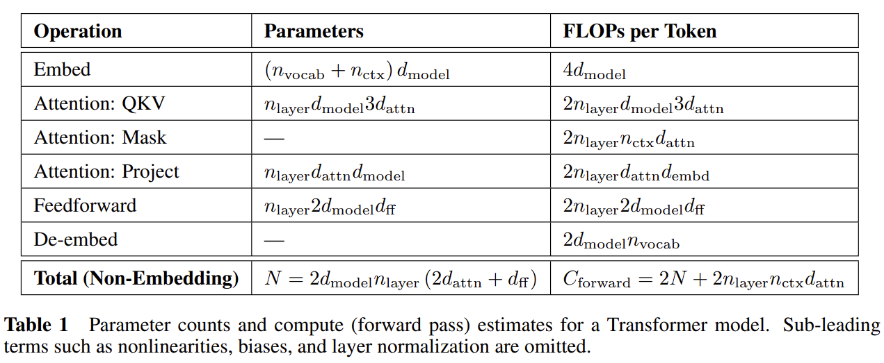
Experimental Results

参考