LLM Scaling Laws 论文摘录 - Scaling Laws for Neural Language Models
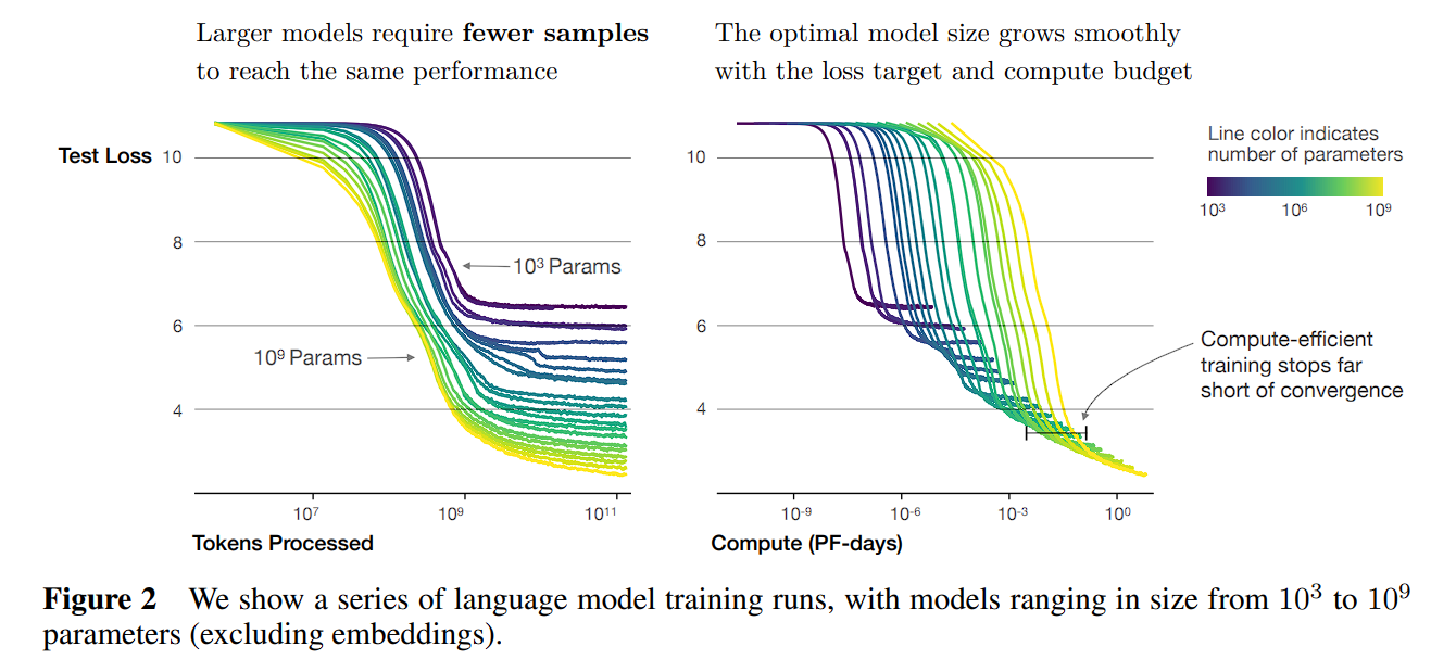
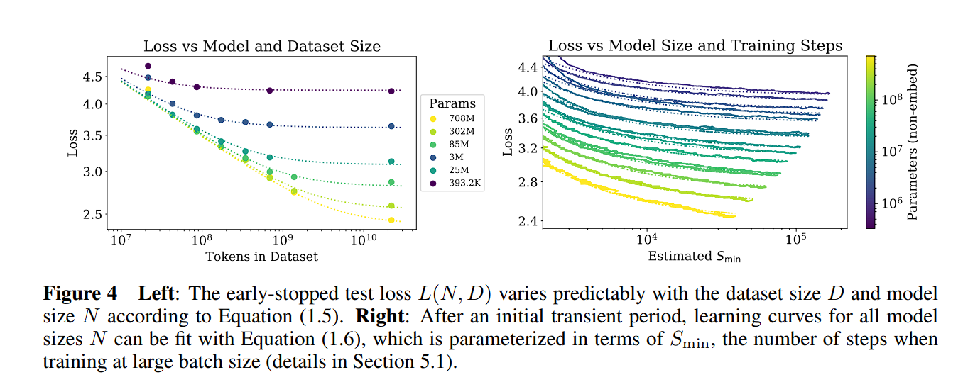
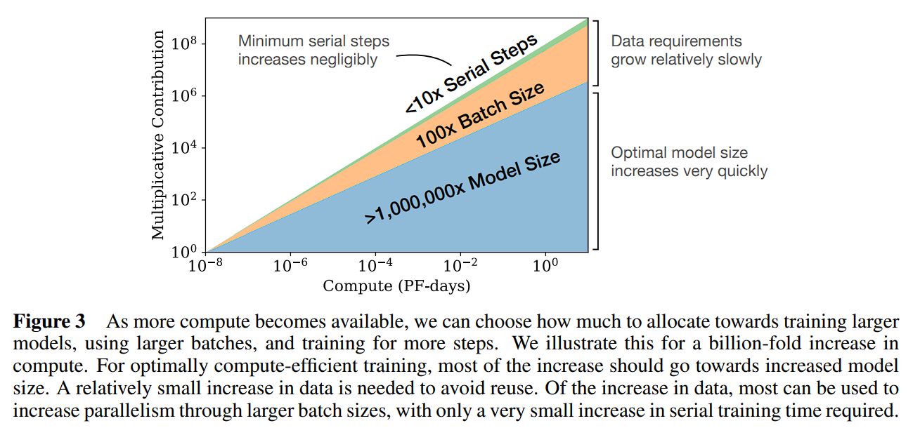
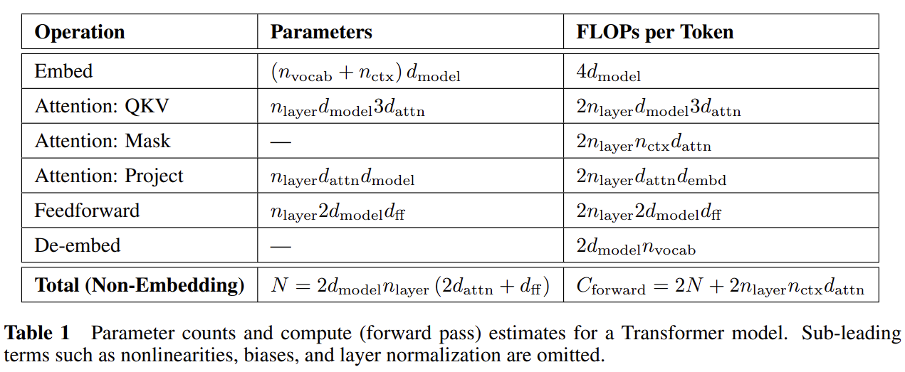
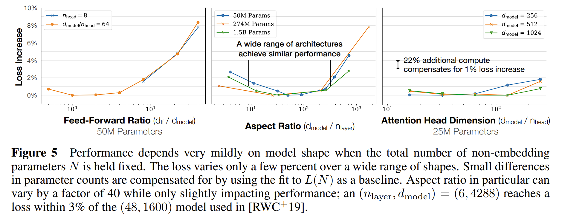
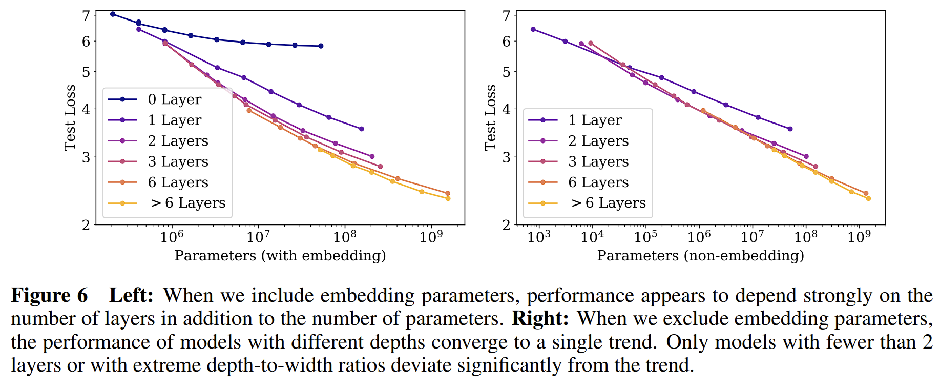
LLM Scaling Laws 论文摘录 - Scaling Laws for Neural Language Models type: Post status: Published date: 2024/03/20 tags: AI, LLM, NLP, 论文摘录 category: 技术分享 OpenAI在2020年发布了《Scaling Laws for Neural Language Models》探讨Scaling Laws(缩放法则),在其中探讨了对于基于Transformerde的大模型的Training Loss与模型参数规模N,数据集大小D,计算量C之间的联系。 而在2022年四月谷歌DeepMind在文章《Training Compute-Optimal Large Language Models》中重新讨论了Scaling Laws,他们指出当前的大模型都明显缺乏足够的训练,在使用四倍的数据(相较于280B参数Gopher)训练70B的Chinchilla后取得了更好的成绩(SOTA average accuracy of 67.5% on the MMLU benchmark, 7% increasement)。 然而,在2023年二月由Thaddée Tyl发布的博客《Chinchilla’s Death》(Chinchilla之死)中,指出,只要训练足够长时间,小模型也能超过大模型。 这张图体现了在相同的计算量大小C的情况下,来自于不同因素究竟有多少贡献。首先是模型大小,其次是数据(通过更大的batch size和减少复用),而Serial Steps(更多的训练次数)帮助并不大 参数: non-embedding parameters $N$ the dataset size $D$ optimally allocated compute budget $C_{min}$ 在其他两因素不受限的情况下,测试损失可以由以下公式预测: $$ \begin{equation} L(N)=(N_c/N)^{\alpha_N} \end{equation} $$ \alpha_N \sim 0.076,N_c \sim 8.8 \times 10^{13} \text{(non-embedding parameters)} $$ $$ \begin{equation} L(D)=(D_c/D)^{\alpha_D} \end{equation} $$ $$ \alpha_D \sim 0.095, D_c \sim 5.4 \times 10^{13}\text{(tokens)} $$ $$ \begin{equation}L(C_{min})=(C^{min}c/C{min})^{\alpha_{min}} \end{equation} $$ $$ \alpha_C^{min} \sim 0.050, C^{min}_c \sim 3.1 \times 10^8 \text{(PF-days)} $$ 公式含义: 在以上三个公式中,$\alpha_N, \alpha_D, \alpha_C^{min}$给出了当我们提升$N,D,C_{min}$时性能提升的幂次。 举个例子,当我们将模型的参数量提升到两倍时,模型的损失将会减小,$2_{-\alpha_N}\approx 0.95$,因此损失将会是此前的0.95倍。而$N_C,D_C,C_C^{min}$的准确数字基于字典大小和tokenization因此没有实际意义,只代表数量级关系。 此外,文章还提到了batch size和loss的关系 $$ \begin{equation}B_{crit}(L)=\frac{B_*}{L^{1/a_B}} \end{equation} $$ $$ B_* \sim 2\cdot10^8 \text{tokens}, \alpha_B\sim0.21 $$ 根据此前公式(1)和公式(2)可以得出,当我们提升模型大小时,我们应相应地增加数据集的数量,可以根据计算得出$D\propto N^{\frac{\alpha_{N}}{\alpha_D}} \sim N^{0.74}$。他们还发现一个结合(1)和(2)的公式来控制N和D的依赖以及控制过拟合: $$ \begin{equation}L(N,D)=\left[\left(\frac{N_c}{N}^{\frac{\alpha_N}{\alpha_D}}+\frac{D_c}{D} \right) \right]^{\alpha_D}\end{equation} $$ 训练的曲线也可以由训练step数得出,因此可以求得最佳训练step数 $$ \begin{equation}L(N,S)=\left(\frac{N_c}{N}\right)^{\alpha{N}}+\left(\frac{S_c}{S_{min}(S)}\right)^{\alpha_S}\end{equation} $$ $S_c \approx 2.1 \times 10^3,\alpha_S \approx 0.76$ $S_{min}(S)$ is the minimum possible number of optimization steps (parameter updates) estimated using Equation 在固定计算量C的情况下,又得出了以下关系公式 $$ \begin{equation}N \propto C^{\alpha^{min}_C /\alpha_N}, B \propto C^{\alpha^{min}_C /\alpha_B}, S \propto C^{\alpha^{min}_C /\alpha_S}, D = B \cdot S\end{equation} $$ 此处有 $$ \begin{equation}\alpha^{min}_C=1/(1/\alpha_S+1/\alpha_B+1/\alpha_N)\end{equation} $$ 可得$N \propto C^{0.73}{min}, B \propto C^{0.24}{min},\text{ and }S \propto C^{0.03}_{min}$,此处提出观点: 研究在数据集WebText2及其拓展($2.29\times 10^{10}$ tokens),tokenize方法为 byte-pair encoding,词汇大小$n_{vocab}=50257$,性能指标(Loss)为在1024个token上下文的中的交叉熵损失。模型使用的是decoder-only的Transformer,同时训练了LSTM和其他类型的Transformer作为比对。 除特别说明外,模型的训练使用了Adam优化器和$2.5 \times 10^5$步,batch size为512,上下文512 token。由于内存限制,最大的模型使用了Adafactor优化器。 除特别说明外,训练的学习率是一个3000步的热身和一个cosine decay余弦衰减到零。 模型的参数计算方法 为了计算模型参数和计算量,模型的超参数定义为: | $n_{layer}$ | 层数 number of layers | | — | — | | $d_{model}$ | 残差流的维度 dimension of the residual stream | | $d_{ff}$ | 前馈层(全连接)的维度 dimension of the intermediate feed-forward layer | | $d_{attn}$ | 注意力输出的维度 dimension of the attention output | | $n_{heads}$ | 每层注意力头数量 number of attention heads per layer | | $n_{ctx}$ | 上下文词元数量,除另说明外为1024 input context | 使用$N$代表模型的参数大小,这里定义为除去embedding的参数: $$ \begin{aligned} N&\approx 2d_{model}n_{layer}(2d_{attn}+d_{ff}) \ &= 12n_{layer}d^2_{model}\end{aligned} $$ $$ d_{attn}=d_{ff}/4=d_{model} $$ 这里省去了embedding层的$n_{vocab}d_{model}$和$n_{ctx}d_{model}$参数,向前传递大概需要计算量$C$如下表示: $$ C_{forward} \approx 2N+2n_{layer}n_{ctx}d_{model} $$ 实验变量: 结论: $$ \begin{aligned} L(N) &\approx (N_c/N)^{\alpha_N} \ L(D) &\approx (D_c/D)^{\alpha_D} \ L(C_{min})&\approx (C_{c}^{min}/C_{min})^{\alpha_{min}} \end{aligned} $$ [1] https://arxiv.org/pdf/2001.08361.pdf [2] https://arxiv.org/pdf/2203.15556.pdf [3] https://espadrine.github.io/blog/posts/chinchilla-s-death.html [4] https://arxiv.org/pdf/2109.10686.pdf [5] https://self-supervised.cs.jhu.edu/sp2023/files/17.retrieval-augmentation.pdfLLM Scaling Laws 论文摘录 - Scaling Laws for Neural Language Models
背景和内容
论文
Scaling Laws for Neural Language Models
主要发现
Scaling Law 总结
$$研究方法
实验结果
Training Compute-Optimal Large Language Models
参考